Hooke’s Law Experiment
Experiment carried out by Lee Ming Loon, student at University of Southampton

Abstract
The main purpose of this experiment is to investigate the behaviour of three different elastic materials. The experiment is carried out for two of the elastic materials which are still within their elastic region while the other elastic material have already exceeded its elastic region, also known as plastic region. The initial length of the elastic material is first measured by using a metre rule. A weight is hung onto the spring and the extension of the elastic material can be measured. The experiment is repeated for different weights. A graph of extension or deformation against the force applied is drawn and the elastic constant of the material can be calculated. The experiment obeys the law of elasticity. The extension of the elastic material is directly proportional to the force applied provided the elastic limit is not exceeded.
Introduction

Robert Hooke was a 17th-century scientist and philosopher who discovered Hooke’s Law which was named after him in 1660. He was born in 1632 in Freshwater, the Isle of Wight, England. Due to Robert’s delicate health as a child, he was kept at home until his father died. When Hooke was 13, he went to London and was apprenticed to painter Peter Lely. He was not bad at art but left because the fumes affected him. He was then enrolled at Westminster School, where he received a solid academic education including wide range of languages and also trained as an instrument maker. Later on, Hooke entered Christ Church college where he invented wide range of things there. The Royal Society for Promoting Natural History caught the attention of Hooke in 1661 after just founded a year earlier and offered him a curator position the following year. Within the next decades, Hooke had contributed to astronomy, microbiology, geometry and many more other fields. Hooke is best known for his identification of the cellular structure of plants. Robert Hooke was died in London in 1703.
Theory
Elasticity is the capability of an object to return to its original shape after the removal of external force. Spring is an example of an elastic material. When a spring is stretched, it can restores to its original length. This phenomenon can be explained by Hooke’s Law.
Hooke’s law is a principle of physics that states that the force needed to stretch an elastic material is proportional to the extension of the material. This can be expressed mathematically by using a graph.
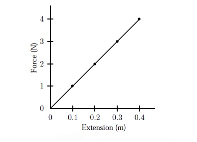
The graph in Figure 1 can be expressed by a formula:
F=kx
where ;
F= the force applied (N)
k= spring constant (N/m)
x= spring extension (m)
This equation is only valid provided the elastic limit is not exceeded. This means that the elastic material will return to its original shape and length without any permanent deformation. If the elastic material does not return to its original shape, it is beyond the elastic limit.
If the force applied to the elastic material is within its elastic limit, there will be a restoring force once the force applied is removed. The restoring force is equals to the force applied but in different direction. Hence, restoring force can be expressed as,
F=-kx
The negative sign (-) is added to signify that the direction of the restoring force is opposite to the force applied to the elastic material.
Spring constant, measured in Newtons per meter (N/m) represent how stiff a spring is. Different spring has different spring constant. The stiffer a spring is, the higher the spring constant. We can calculate the spring constant by using the formula k=F/x or simply find the gradient of the line from the graph.
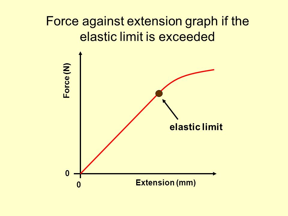
When the material exceeds its elastic limit, the graph will not look like the graph in Figure 1. It will be a straight line anymore but it will starts to curve. The graph will looks like below in Figure 2.
Method
Three different elastic material, material 1 (y1), material 2(y2) and material 3 (z) is prepared. The initial length of these three material is measured and recorded.
Material 1 (y1) is first hung onto the retort stand. A mass hanger which weight 1N is hooked to the spring. The final length of material 1 is measured and recorded. The experiment is repeated with eight more different masses which weight from 2N to 9N by adding slotted mass (1N) onto the mass hanger. The final length for each of the weight is measured. The extension of the material can be calculated by using the following formula:
Extension = Final length – Initial length
The extension of the material is tabulated to a table.
The entire experiment is then repeated using material 2(y2) and material 3 (z) respectively. After all the measurements obtained from the experiment have been tabulated to a table, a graph of extension against force applied to the material is plotted. A line of best fit is drawn if the material obeys Hooke’s Law.
Results and Discussion
| Force applied, x (N) | Extension of material 1, (y1) | Extension of material 2, (y2) | Extension of material 3, z |
| 1.00 | 3.00 | 2.26 | 2.38 |
| 2.00 | 4.50 | 4.32 | 9.38 |
| 3.00 | 6.00 | 6.37 | 28.38 |
| 4.00 | 7.50 | 8.43 | 65.38 |
| 5.00 | 9.00 | 10.49 | 126.38 |
| 6.00 | 10.50 | 12.55 | 217.38 |
| 7.00 | 13.00 | 14.61 | 344.38 |
| 8.00 | 14.00 | 16.67 | 513.38 |
| 9.00 | 15.00 | 18.72 | 730.38 |
Table 1. Value of extension of Material 1 (y1) , 2 (y2) and 3 (z) after a force is applied.
The formulae of y1 , y2 and z are given. The formulae are shown below:
y1 = ax + b
y2 = (a + 0.5)x+ c , where c = 0.2
z = x3 + b
The values of a and b can be found from Graph 1.
a is the gradient of the trend line and b is the intercept of vertical axis.
From Graph 1,
a = 1.5583
b = 1.375
Hence,
y1 = 1.5583x + 1.375
y2 = (1.5583 + 0.5)x+ 0.2
z = x3 + 1.375
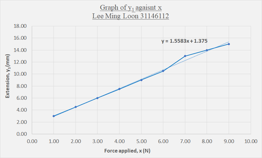
Graph 1 is a linear graph where the extension of material 1 (y1) is directly proportional to the force applied. This means material 1 (y1) obeys Hooke’s law and is within the elastic limit and will return to its original length after the removal of force.
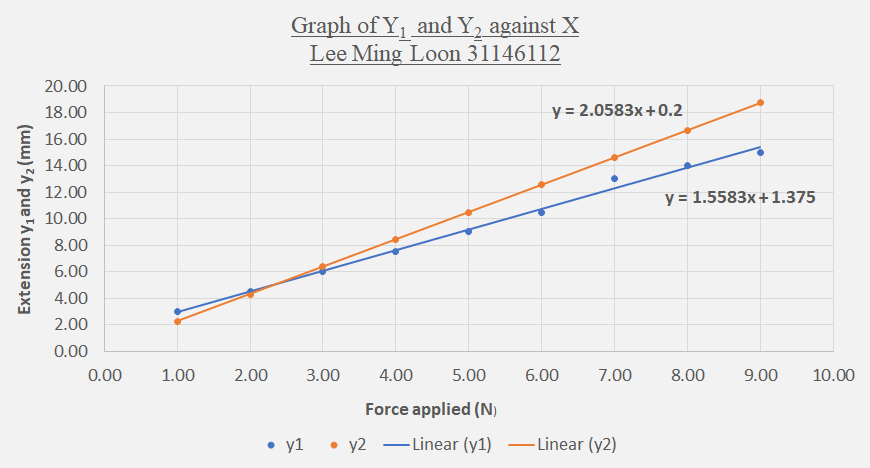
Both of material 1 (y1) and material 2 (y2) is plotted above in Graph 2. We can see that material 2 (y2) is also a straight line. Hence, it obeys Hooke’s law. Same as material 1, the extension of material 2 is directly proportional to the force applied and it will restores its original length when the force is released.
Besides that, we can compare the steepness of two lines in Graph 2 to differentiate which material has a higher spring constant. The material with a greater spring constant is stiffer and less elastic. So, we can calculate the gradient of the line of each material to know which line is steeper.
We can calculate the spring constant by rearranging the formula of Hooke’s law, and we get:
k=F/x
Another way of calculating the spring constant is simply finding the gradient, m of the graph of force applied against extension. However in Graph 2, the graph is plotted extension against force applied. Therefore, the spring constant can be obtained by calculating the reciprocal of the gradient,m on the graph for each material.
The formula of gradient is : (Y2– Y1)/(X2– X1)
Gradient of material 1, m1= 1.5583
Spring constant, k1 of material 1 = 1/1.5583
= 0.6417 N/mm
= 641.7 N/m
Gradient of material 2, m2 = 1.5583
Spring constant, k2 of material 2 = 1/2.0583
= 0.4858 N/mm
= 485.8 N/m
Since k1>k2 , this proved that material 1 is stiffer than material 2. In consequence, a greater force is required to stretch material 1 to the extension as material 2.
As we can notice that there is an interception point between the two lines on the graph. The point of interception can be found by solving the simultaneous equations of the two lines which are y=2.0583x+0.2 and y=1.5583x+1.375. We can also find the interception point in Microsoft Excel by using matrix. The formula for this method is:
MMULT(MINVERSE(A),B)
where;
A= values of x and y
B= value of c
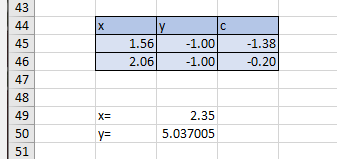
For the table above, we can find x value by using the formula:
MMULT(MINVERSE(B45:C46),(D45:D46))
We get the value of x interception which is 2.35N
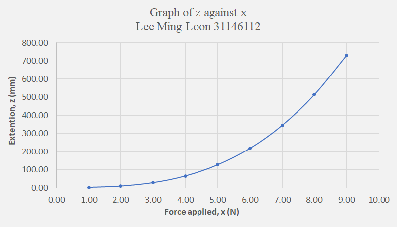
Graph 3 is a exponential graph. Since it is not a linear graph, we cannot say that material 3 (z) is a elastic material. Material 3 does not obey Hooke’s law, it will not return to its original shape and length after a force is applied on it. We can say that material 3 is undergoing a permanent plastic deformation.
Conclusion
We can conclude the characteristic of these three materials. Material 1 (y1) and material 2 (y2) are elastic material as they obey Hooke’s law. We can also define from Graph 2 that material 1 (y1) is stiffer and less elastic than material 2 (y2) due to greater spring constant, k. Lastly, material 3 (z) is considered an inelastic material because Graph 3 is an exponential graph rather then a linear graph. It undergoes plastic deformation and will not return to its original length and shape after a force is applied.
However, errors could happen in the experiment and must be taken into consideration. For example, the line in Graph 1 does not pass through the origin (0,0). Also, the lines in Graph 2 should not intercept each other. These errors are probably due to systematic error. For example, the mass hanger and slotted mass may not weight exactly 1N. Human error is one of the reason as well. Metre rule may not be placed at one of the end of the material at the 0m mark scale when measuring it. Furthermore, there may be parallax error when reading the scale. Parallax error means that the level of eye is not perpendicular to the scale of the metre rule.
References
Marry Bellis, (2019). Biography of Robert Hooke, the Man Who Discovered Cells [online] Available at: https://www.thoughtco.com/robert-hooke-discovered-cells-1991327
Matt Williams, (2015). What is Hooke’s Law? [online] Available at: https://phys.org/news/2015-02-law.html
Khan Academy, (n.d.). What is Hooke’s Law? [online] Available at: https://www.khanacademy.org/science/physics/work-and-energy/hookes-law/a/what-is-hookes-law [Accessed 30 October 2019].
Follow My Blog
Get new content delivered directly to your inbox.
